this is designed for the about link on the homepage to auto expand
Dot Product
Introduction
So this isn't actually a physics lesson. Like the vectors section, it's intended to brush up on external concepts that will prove to be essential to the later discussion of physics concepts. This lesson will focus on the concept of dot product, an operator of vector algebra. It's one of the two ways vectors can be multiplied together. (Incidentally, the other method is also pretty widely used in physics, but only in rotational dynamics and electromagnetism.)
The dot product somewhat describes the projection of one vector onto another. It's denoted with a big old dot like this: $\vec{a} \cdot \vec{b}$. More accurately, it technically better describes how parallel or orthogonal (perpendicular) two vectors are to one another, with a value of one meaning the vectors are entirely parallel, a value of zero meaning the vectors are orthogonal, and a value of negative one meaning the vectors are antiparallel. Notice how these values are all scalars! Indeed, the dot product takes two vectors and outputs a scalar quantity. I'll take two arbitrary vectors to show you how this operator works.
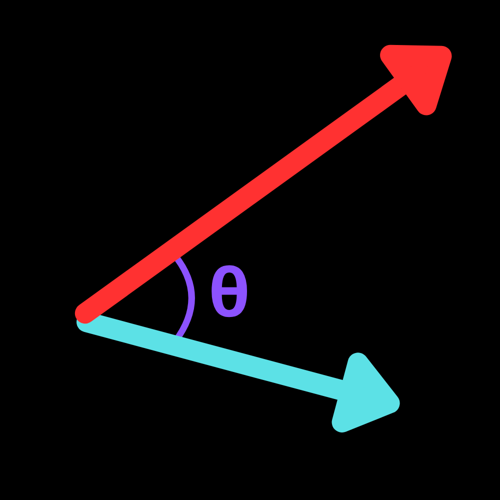
Figure 1: Two unsuspecting vectors we'll use as our test subjects.
Formula
Unlike adding or subtracting vectors, with the dot product there is no real way to perform it graphically. (This makes sense, since you're outputting a scalar and we don't typically represent scalars on graphs.) The first way to do so is to use the magnitudes of the two vectors, which we'll call $\vec{a}$ and $\vec{b}$ as well as the angle $\theta$ between the two. In that case, the dot product is defined as:
$$\vec{a} \cdot \vec{b} = |\vec{a}|~|\vec{b}| \cos \theta$$ Let's break this down a little bit. I'm mainly just interested in the cosine part, since the two vectors are arbitrary. Now, we know that cosine takes a range of values $-1 ~\leq \cos \theta ~\leq 1$. The cosine is equal to one and negative one when the vectors are parallel and antiparallel, respectively. This matches up with what I talked about before. Additionally, if the angle $\theta$ is a right angle, then the cosine is zero and the dot product evaluates to zero, which matches the orthogonality condition I touched on briefly.
Any values between these will evaluate to something (with an absolute value) less than one but greater than zero, which covers all of the cases where the vectors aren't perfectly parallel or perpendicular. Vectors that are more parallel will have a smaller angle $\theta$ between them, which evaluates to a higher value of cosine and vice versa. So, with just a bit of analyzing a basic trig function (which you should know how to do), we have de-mystified the dot product.
Isn't that nice and simple? While in math this form is rarely used, it's much more common in physics. There's also one key takeaway from this equation. This tells us that the dot product is equal to the component of $\vec{a}$ on $\vec{b}$ multiplied by the magnitude of $\vec{b}$. You'll see how important this is later on.
Just presenting one form of this operator is a bit limiting, however. Therefore, I'll be showing the other algebraic way to compute the dot product even though it's less useful for physics. The dot product basically tells us how much of one vector "fits" onto another. It basically tells us how parallel or perpendicular the two vectors are, with a greater value meaning more parallel vectors. A negative value means the vectors are pointing in opposite directions (antiparallel). Let's use a diagram to illustrate the basic math about this operator:
Figure 1: Two unsuspecting vectors we'll use as our test subjects.
Formula
Now, this part requires a bit of trig knowledge. Remember our vectors lesson, and the idea of components. To get the component of any of the two vectors on the other, the function we want to use is the cosine. This allows us to have an intuitive understanding of why the dot product formula is what it is. Enough suspense, here it is:
$$\vec{a} \cdot \vec{b} = |\vec{a}|~|\vec{b}| \cos \theta$$ The dot between the two vectors denotes the dot product. (It's called dot product for a reason.)
We can analyze this function by analyzing the cosine function, but this might be a bit too mathematical. Instead, we're just going to recognize that the cosine can range from negative one to one, allowing for a range of values for the dot product. Moreover, the dot product is really just equal to the product of the component of $\vec{a}$ on $\vec{b}$ and the magnitude of $\vec{b}$. This will come in handy for physics problems.
This is really enough knowledge of the dot product for physics, but for the sake of having a thorough lesson let's talk about the other way to write the dot product.
The other form of the dot product requires the use of vector components. While in physics you're more commonly given the angle between two vectors of interest, in math you're mostly given vectors in component form. Additionally, it's not unheard of to give vector components in physics, so it'll be good to know this second form of the dot product.
Alternative Methods
This form of the dot product is arguably simpler than the first. I'm going to use the standard notation for components with subscripts that designate the dimension. In a 2D form, it can be written as:
$$\vec{a} \cdot \vec{b} = a_xb_x+a_yb_y$$
In 3D, it takes a very similar form:
$$\vec{a} \cdot \vec{b} = a_xb_x+a_yb_y+a_zb_z$$
This isn't too complex, is it? This method of computing the dot product is far more convenient when you're given the components, and is widely used for problems in 3D because vectors in those cases are most often expressed in terms of their components for convenience.
In fact, while the first method of computing the dot product would technically work here, it would only be convenient for vectors that were in a convenient plane (finding the angle would otherwise be hard). I'm not even sure if it would work in 4D or higher, since those dimensions are impossible to visualize. In any case, this new form can be generalized to any number of dimensions:
$$\vec{a} \cdot \vec{b} = \sum a_i b_i$$
The letter $i$ denotes each individual dimension, and we simply sum the product over the total number of dimensions. While in the physical world there are only three dimensions (actually, there might be 11, but that's WAY out of the scope of what we're talking about here), using vectors can allow for mathematical shortcuts and the "extra" dimensions are often used in calculations. But we'll be sticking to three dimensions max.
With that, let's dive into a simple example that utilizes this method.
Find the dot product of two vectors $\vec{o} = \langle 3, 12, -1 \rangle $ and $\vec{p} = \langle -4, 0.5, 2 \rangle$.
This is just a direct computation with the formula given before.
This is definitely the easier of the two vector products, involving pretty straightforward calculations. This lesson was pretty short as a result, but you still need to make sure that you're clear on how the dot product works. Why? The next lesson will cover our first physics concept of this unit, which coincidentally relies on the dot product! I wonder why that is...